Conclusion and Extension to Higher Dimensions
We've gone through a long journey, haven't we? It's time to wrap it up.
First, we introduced the problem of not knowing further information about a stable point, in particular, not knowing whether it's a maximal point, a minimal point, or a saddle point.
Then we figured out a useful way by taking the quadratic approximation of the function, transferring the problem to whether the stable point is a maximum, minimum, or saddle point on the quadratic approximation.
Then we've concentrated on the most insightful part of the quadratic approximation, which is simplified to be , where and . We extracted the Hessian matrix, left out the constant , and got . After finding out that the matrix has two eigenvalues and eigenvectors that are perpendicular to each other, we took the two orthogonal unit eigenvectors as new basis vectors in a new coordinate system, and changed the basis of into them. As a result, we got:

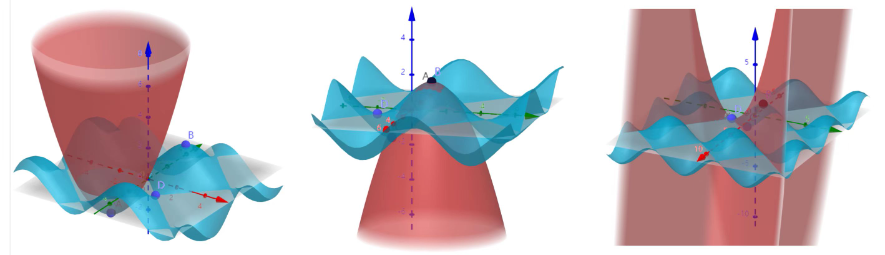
, where and are the corresponding eigenvalues of the eigenvectors, and is the coordinates of a point under the new coordinate system. The term is interpreted as stretching the along the vertical direction on the z-m plane by a factor of and the along the vertical direction on the z-n plane by a factor of , which is why the quadratic approximation function is symmetric with respect to both the z-m plane and the z-n plane. Play around with the visualization below again if you like.
So we know if the eigenvalues and , the point or is a minimal point on , thus a minimal point on the quadratic approximation:
, and thus a local minimal point on the original function.
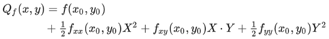
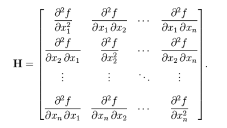
Likewise, we can conclude that if and , we get a local maximal point and if , a saddle point. The eigenvalues and basically tell us the shape of the quadratic approximation.
In a higher-dimensional case with more than two inputs, however, things get difficult to visualize. But following the same idea, all we have to do is to analyze the eigenvalues of a Hessian matrix at a stable point, in order to identify it as a local maximum, local minimum, or saddle point.
The Hessian matrix at a stable point includes all the second-order derivatives of a function at this stable point, written as:
We then compute its eigenvalues, which is often not very easy a task and is often left to the computer. So suppose we have the eigenvalues in our hands. Because their corresponding eigenvectors are all perpendicular to each other (the proof of this also gets harder, you can google it if you like), the quadratic approximation of our original function at a stable point should be under the new coordinate system made up of all the unit eigenvectors. Then all we have to do is to check the eigenvalues' positivity and negativity. If they are all greater than 0, then all the points on the quadratic approximation are above the stable point, thus our stable point is a local minimum. If they are all less than 0, then we get a local maximum. If at least one is negative and at least one is positive, we get a saddle point.
P.S.
1. Using this method gives out only the local minimum or maximum of a function, not the global ones.
2. The special cases where the stable point is neither a maximum, a minimum, nor a saddle point are not discussed, for example when one of the second-order derivatives is 0. You could think about them if you like.
3. If you've gone so far as to finish reading this article, I would very much love some feedback! Since geogebra doesn't seem to have a place for comments, here's a link to a discussion on Discord.
https://discord.com/channels/834837272234426438/1142042947156705282
Feel free to share your ideas!