Quadratic Approximation in Multivariable Case
We know from the single variable case that we can calculate the quadratic approximation of the function at a stable point, to find out whether it's a maximum or minimum. Now let's apply the same method to our two-variable case.
Alter variables a and b to alter point A. Observe how the quadratic approximation changes. There are 3 given stable points in the graph.
As we see above, the shape of the quadratic approximation is pretty close to the shape of the function at the stable point. So if this point corresponds to a minimum in the quadratic approximation, it should be a local minimum on the function. Likewise, we could identify maxima and saddle points.
Extending the case of the single variable function, a quadratic approximation of a multivariable function at some point satisfies the following properties:
1. is a quadratic function;
2. goes through this point;
3. its first-order derivatives at this point with respect to each variable is equal to the function's;
4. its second-order derivatives at this point with respect to each variable is equal to the function's.
First, we have to introduce the second-order derivatives of a multivariable function. Again, if that is contained in your background knowledge, skip to "So the quadratic approximation...".
You might have guessed there are two second-order derivatives for a two-variable function, which are the ones with respect either to or . Yes, this is true, and the clever you may have already guessed the meaning of them. They are the second-order derivatives of the intersection curves, which we sliced out from the function (the curved surface) like in the first chapter. When taking the second-order derivative of with respect to , we consider the variable to be a constant, so the result is . And the second-order derivative with respect to is .
Function sliced by the planes x=a and y=b.
But this is not enough. The quadratic terms in the quadratic approximation should be in the form of (p, q, and t are constants). Here, if we take the quadratic approximation at point , we know that and . What about the ? This term indeed contributes significantly to the shape of our quadratic approximation. You could try this out by changing the value of while keeping and constant in the red graph below.
But is canceled out when you take the second-order derivative of with respect to either or . is only reserved when you first take the derivative with respect to then with respect to . In the original function, the derivative with respect to then happens to be 0, so here . By the way, for any function, taking the derivative with respect to then is always the same as first to then . You can try this out with an arbitrary function you think of.
The second-order derivatives are written as , and .
So the quadratic approximation of at , is:
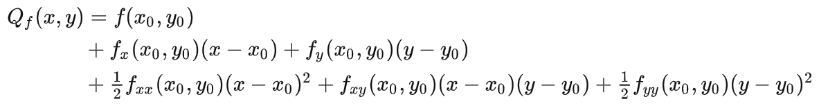
Verify that this quadratic approximation satisfies all the properties it should have.
Indeed, this formula seems terrifying at first glance, but we could significantly simplify it by realizing that the first-order derivatives at a stable point are all zero, and by letting and .
So the quadratic approximation of of at a stable point is just:
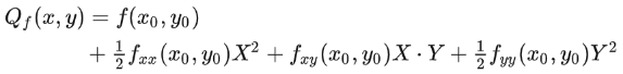
This is still a bit intimidating, but notice that , and are all just constants given the point , so we can assume them to be , , and . That leaves us with:
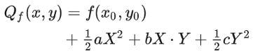

Now, we'd like to identify the stable point either as a maximum, a minimum, or a saddle point. This is the same as figuring out whether all the other points on the quadratic approximation are below the stable point, above the stable point, or both at the same time. So all the trouble reduces to comparing the term with 0.
Alter the variables a, b, and c to see the result.
As you might notice, when is 0, it's quite easy to know whether the quadratic term is positive or negative just by looking at the values of and . You could try to reason this yourself.