Algorithm for finding the expected locations of Local maxima, minima or saddle points of stationary points of a numerical function of two variables in the coordinate descent-ascent method
As a numerical function, we consider the intensity distribution of the diffraction field when light is diffracted by a single slit: J=J(x,y). The order of operations is the same as for the explicit set function discussed in applet 1. The algorithms for finding max / min can be found in applet 2, and the algorithm for finding a saddle point can be found in applet 3. The applet of the proposed coordinate descent-ascent algorithm for computing stationary points of a numerical function can be found in 4.
A method is proposed to find the conditional extrema of an numerical function of two variables J(x,y) by gradually approaching the target and changing the values of the X and Y sliders indicating the corresponding coordinates. The case of the distribution of the diffraction field, i.e. the intensity J(x,y), behind the slit is considered.
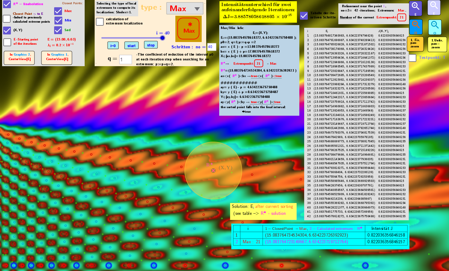
The search for the type of extremum is performed by selecting the max/min/sad option in the applet. To select the starting point of the iteration E and to estimate the accuracy of the calculations performed, the Heatmap of the dependence J(x,y) is specified, as well as the distribution of the extremum points previously calculated by another method (as ClosestPoint). The point E should be entered in the area of the region of interest, which is represented in the applet as a circle with radius p0. In another window on the left, this area can be centered and zoomed using the buttons provided. By clicking the button i=0 and starting the animation, the iterative process begins, which you can observe. You can judge the convergence process by ΔJ, how two successive values of the surface function are related to each other at two approximation points. It happens that at the beginning of the iterations there are no successive changes - it is necessary to change the starting point E or the search radius p0. The environment of the point E must contain the expected extremum (stationary point). Otherwise there is no convergence. In the considered case of numerically defined function, as it turned out, the most productive variant was the case of constant width of the search interval: po-const, i.e. q=1.
General view of the applet for the case of saddle point search
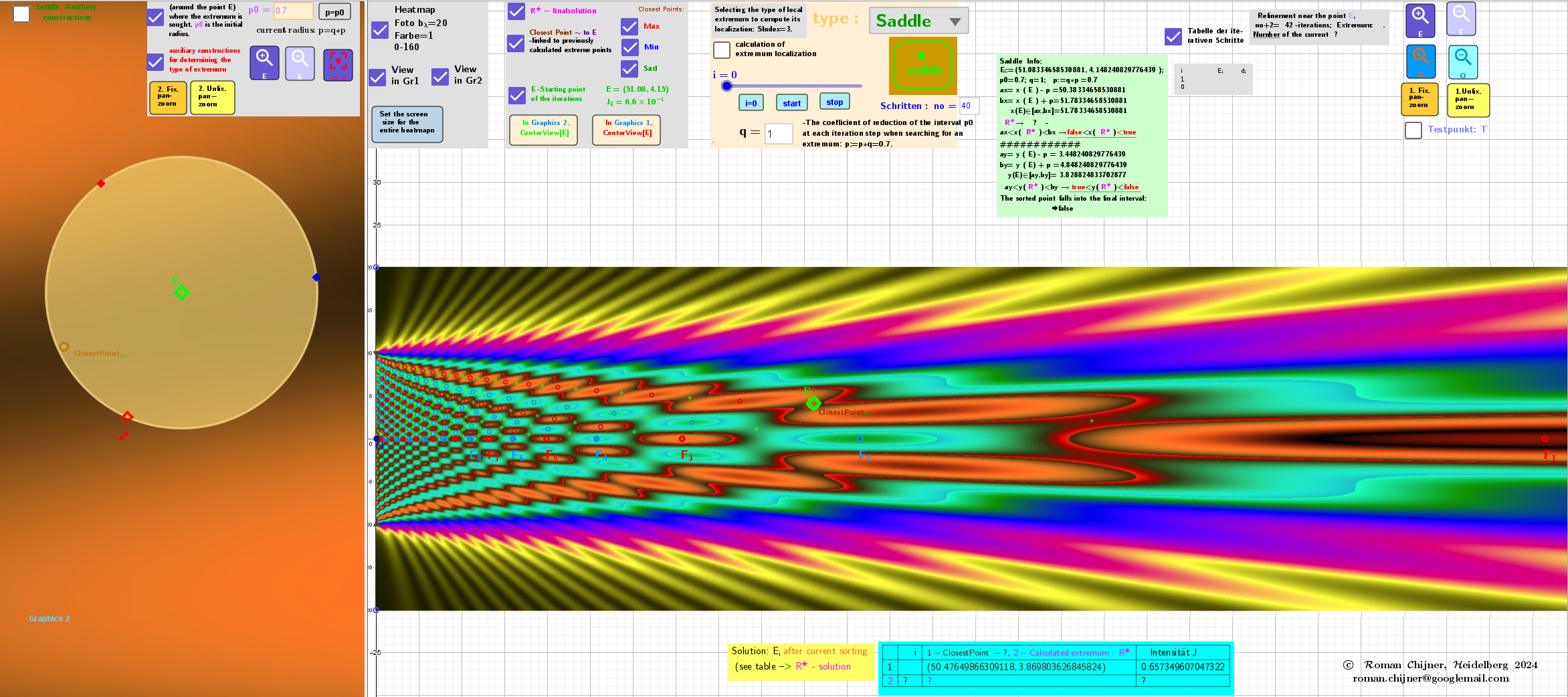
The starting point E and the moving point (X, Y), whose coordinates are the corresponding X and Y sliders on the Heatmap in the search area using iterations

Positions of sliders (X,Y) and table after iterations. R* is the final localization of the desired stationary point.
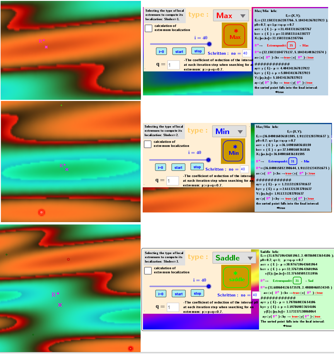
Examples of individual cases of the calculation of stationary points in the applet: possible Local maximum, minimum and saddle point