Interpreting the Hessian Matrix to Identify a Stable Point
We've so far transferred the problem of identifying a stable point as a minimum, maximum, or saddle point to determining whether the term is always positive, negative, or sometimes positive and sometimes negative.
If you know some matrix multiplications, you'll be able to see that the term above is equal to:
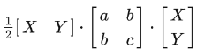
And according to how we defined , , and before, , which is exactly what the Hessian matrix is in the two-variable case. But we'll just leave it to , , and for the sake of concision.
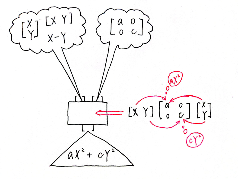
So, if we ignore the factor temporarily (because it does not change the term's positivity or negativity), we get . But what does this actually mean? In the simpler cases, where b equals 0, we have . Imagine the process going on here as this: there are two inputs, one is our diagonal matrix (a matrix in which the entries outside the main diagonal are all zero), the other is our X-Y coordinate system. Our algorithm then spits out a function, the height for every point .
Alter a and c and observe the shape of the curved surface from different angles.
I hope you would get an intuition of what a diagonal matrix is really doing to the coordinate system. It is not operating the X-Y plane by stretching the X-axis by a factor of and the Y-axis by a factor of . Instead, if you think of the initial value as , the matrix stretches the on the z-X plane along the vertical direction by a factor of and the on the z-Y plane by a factor of , thus giving out . And that's why the curved surface is symmetric both with respect to the z-X plane and with respect to the z-Y plane. Check this by observing the function from top to down.
It's obvious that is always true, and so is , while can be both positive and negative. So extending this idea, we can conclude that:
If and , then the stable point is a minimal point.
If and , then the stable point is a maximal point.
If , then the stable point is a saddle point.
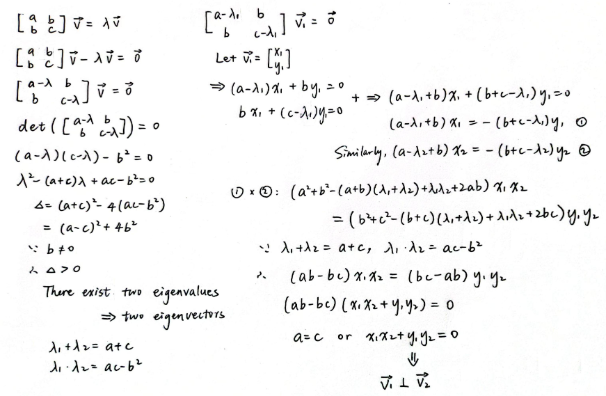
We are finally getting to the complicated case where is not zero. There's this matrix as our input, but we don't really understand what it's doing. Why not change it into a diagonal matrix? That's the fundamental idea behind the eigenvalues and eigenvectors. A quick reminder: if an eigenvector is , and its corresponding eigenvalue is , we'll have , which means that the only thing the matrix does to the eigenvector is stretching it by a factor of . Computationally, we can prove that there exist two eigenvalues and that the two eigenvectors are perpendicular to each other. I'll leave the proof below. If it does not interest you, you can skip that and just keep the two conclusions in mind.
Because the two eigenvectors are perpendicular to each other, we can choose them so that they look just like rotating the unit vectors and in the X-Y coordinate system by degrees. (Let be rotated 90 degrees counterclockwise.)
You can alter θ.
Now, we can change the basis of our matrix into the two unit eigenvectors and . As we see above, , . Putting them into a matrix, we get , which transforms the original basis vectors and into and , and which is just a rotation matrix of degrees.
Applying the change of basis, we know . Why is this true? (If you already understand the change of basis, skip to "We're almost there".) First, is the inverse matrix of , which means applying it should transform the new basis vectors and back to the old ones and . If you displace yourself into the position of the new coordinate system made up of and , you'll think that and , which is where you want your basis vectors to go. So you put them into the columns of a matrix, and get, which transforms your basis and back to and .
Or maybe you'd like to think of it in another way. The inverse of is just rotating back the basis vectors by degrees, which is a rotation by degrees. So the inverse matrix is just .
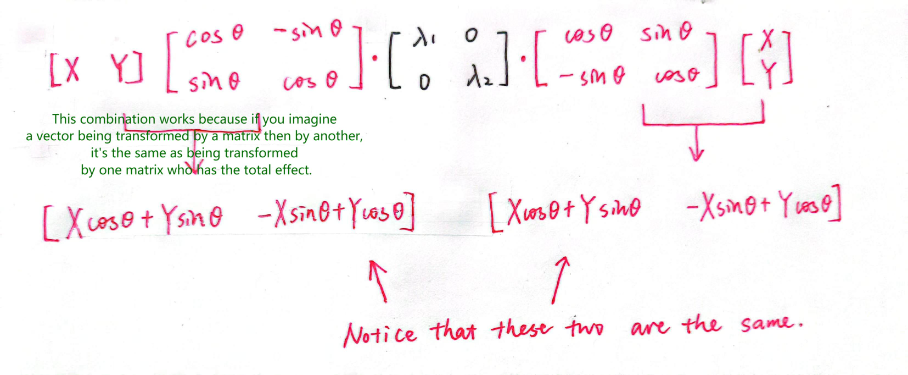
The change of basis includes viewing a linear transformation from different perspectives. Under the new coordinate system, we have the matrix, but a new coordinate system which has and as its basis vectors would think that it was put under a linear transformation of, its coordinate axes each stretched by the corresponding eigenvalue. We now interpret the latter one. Let's say you want to know the coordinates of in the new coordinate system, assuming it to be. Then, from the perspective of your new coordinate system,. Next, the new coordinate axes are each just stretched by some factor, giving us, which is where our observed vector lands up, say at, however in the language of your new coordinate system. The old coordinate system would rather think of it as . Multiplying all this bunch of things together, we get where lands up after the linear transformation,, which is exactly the same as . Therefore we've now understood the equation.
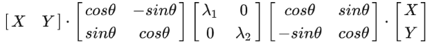
We're almost there. Remember that we were trying to figure out whether the term is positive or negative? We now translate it into the coordinate system made up of its eigenvectors, to bring in a diagonal matrix that we are perfectly comfortable with:
This looks very symmetric.
If we let and. We shall see that:

Is this familiar to you? Under the new coordinate system (in which the coordinate axes are still perpendicular to each other), the function can be rewritten as , where we have as the -axis and as the -axis. The on the z-m plane is stretched along the vertical direction by a factor of , the on the z-n plane by a factor of . Also, the curved surface is symmetric with respect to both the z-m plane and the z-n plane (observe the function from top to down).
Alter a, b, and c and see what happens. Keep an eye on the eigenvalues lambda. (The lambdas are under the function f(x, y) in the left column. I somehow couldn't put it into the graph. Sorry about that.)
So the conclusion is:
If and , then is always true, thus the stable point is a minimum.
If and , then is always true, thus the stable point is a maximum.
If , then can both be negative and positive, thus the stable point is a saddle point.