Angles

Autor:Rafael Losada Liste

This activity belongs to the GeoGebra book GeoGebra Principia. The following is one of the images generated using the dynamic color scanner that I particularly like. The scanner has tremendous versatility, it can create a heat map for virtually any situation [3, 19, 26, 27, 31].

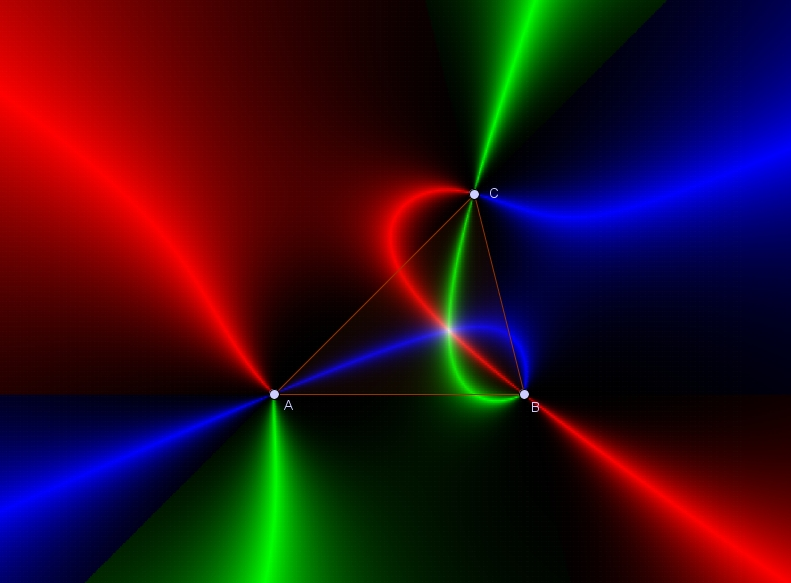In this case, the first isogonic point I₁ is visualized by intersecting the loci that see each pair of sides of the triangle under the same angle.

Note: I₁ coincides with the Fermat point when the triangle's largest angle is not greater than 120º; otherwise, the Fermat point coincides with the vertex corresponding to that angle. It can be calculated directly as the triangle's center X(13) :

I₁ = TriangleCenter(O, A, B, 13).

However, constructing the scanner takes some effort. But we can use CAS to define not only distances but also angles. If someone still thinks that using the expression XA instead of sqrt((x − x(A))² + (y − y(A))²) doesn't save much work, perhaps they'll reconsider now when they can use the expression OXA, defined in the CAS view as: OXA(x,y):= Angle(O, X, A) instead of its algebraic equivalent (with O=(a,b) and A=(c,d)):

cos^–1((a c – a x + b d – b y – c x – d y + x² + y²) sqrt(a² c² – 2a² c x + a² d² – 2a² d y + a² x² + a² y² – 2a c² x + 4a c x² – 2a d² x + 4a d x y – 2a x³ – 2a x y² + b² c² – 2b² c x + b² d² – 2b² d y + b² x² + b² y² – 2b c² y + 4b c x y – 2b d² y + 4b d y² – 2b x² y – 2b y³ + c² x² + c² y² – 2c x³ – 2c x y² + d² x² + d² y² – 2d x² y – 2d y³ + x⁴ + 2x² y² + y⁴) / (a² c² – 2a² c x + a² d² – 2a² d y + a² x² + a² y² – 2a c² x + 4a c x² – 2a d² x + 4a d x y – 2a x³ – 2a x y² + b² c² – 2b² c x + b² d² – 2b² d y + b² x² + b² y² – 2b c² y + 4b c x y – 2b d² y + 4b d y² – 2b x² y – 2b y³ + c² x² + c² y² – 2c x³ – 2c x y² + d² x² + d² y² – 2d x² y – 2d y³ + x⁴ + 2x² y² + y⁴))

Naturally, this expression is merely a development deduced from the dot product of two vectors: vO(x,y):= Vector(X, O) vA(x,y):= Vector(X, A) OXA(x,y):= acos((vO vA)/(|vO|*|vA|)) The significant advantage, besides convenience, is that the Angle command allows us to explore angular relationships without needing to know even the basic operations with vectors, like the dot product. Here, we can see, for example, the locus corresponding to points that form an angle (in radians) equal to the distance to point A with segment OA: OXA – XA = 0

Note: Circles whose arcs span an angle OXA equivalent to XA radians have centers:

(O + A)/2 ± PerpendicularVector(OA)/(2 tan(XA))

And those that see segments OA and OB from the same angle: OXA – OXB = 0 Finally, the intersection of this latter locus with the one corresponding to the equation OXA – AXB = 0 is the sought-after Fermat point.

Author of the construction of GeoGebra: Rafael Losada.

Angles

Novos Materiais

Descobrir recursos

Explorar Tópicos