Field and Current Layers in a doubly fed slip-ring asynchronous machine
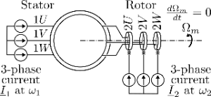
In this animation the rotor (2) and stator (1) are fed by a controllable (in phase, frequency and amplitude) three phase current and the rotor speed follows from the slip equation: with the number of pole pairs ( in the animation). Note also that for phase belt 1U and 2U are in line when (with the rotor angular displacement at ). is assumed so that the motor torque is always equal to the load torque : (i.e. only steady state conditions are animated).
Red and pink waveforms are the current densities and (A/m) of stator and rotor respectively. It is assumed that the phase conductors are spread very finely/thin over the phase width (), so that the current density is a constant over a phase width.
The black waveforms (dashed line) and (dash-dot line) are the accompanying mmfs (Aw) produced by the current densities and respectively (where and symmetry requirements allow to locate the neutral point where ). Please see also: https://www.geogebra.org/m/azhgwttv and https://www.geogebra.org/m/tny9ykfg.
The solid black line is the total mmf of rotor and stator, .
The torque resulting from a rotating fundamental field layer and rotating fundamental current layer can be calculated with . In this animation the reluctance of the iron core is neglected so that the air-gap induction in each point of the armature circumference follows directly from the local total mmf of rotor and stator: with and the air gap length. The torques and (produced by the fundamental functions) are given by [Nm]: and with some (machine) constant. In the animation the torques are then given in relation to the maximum attainable torque in the animation [pu].
Field orientation can be achieved when:
- the fundamental parts of and are in phase, or
- the fundamental parts of and are in phase