Descent-ascent numerical method for finding the stationary points of a function of two variables without using its derivatives. 3.3
f(x,y)=kf (3ℯ-(y + 1)² - x² (x - 1)² - ℯ-(x + 1)² - 8² / 3 + ℯ-x² - y² (10x³ - 2x + 10y⁵))
*The applet will work at a much faster speed if you download it to a desktop computer.
The order of operations for computing stationary points can be found in the applet.
Interactively find and compute local extrema of a nonlinear function of two variables without using its derivatives.
Under the applet, you will find the stationary points of the function in question, calculated on a desktop computer, and you can compare them with more accurate calculations in CAS based on knowledge of the analytical formulas for its partial derivatives.
The iteration process consists of no+2 steps. When searching for local maxima and minima, the function values of the iteration points are sorted for all steps. However, such sorting is difficult because these values coincide within the accuracy of the GeoGebra algebra. Therefore, to find the largest/smallest value, this sorting is additionally performed in GeoGebra CAS with higher accuracy.
To calculate saddle points, di - the distance between two characteristic points for each iteration - was chosen as a criterion. The iteration is considered optimal if this distance is minimal. These distances for different iterations differ enough that the calculations can be done without using CAS.
*Explanations of the algorithms for searching for stationary points can be found in the applets 1 and 2.
Implicit curves of the equations: fx(x,y)=0 and fy(x,y)=0. Contour lines. Location of stationary points
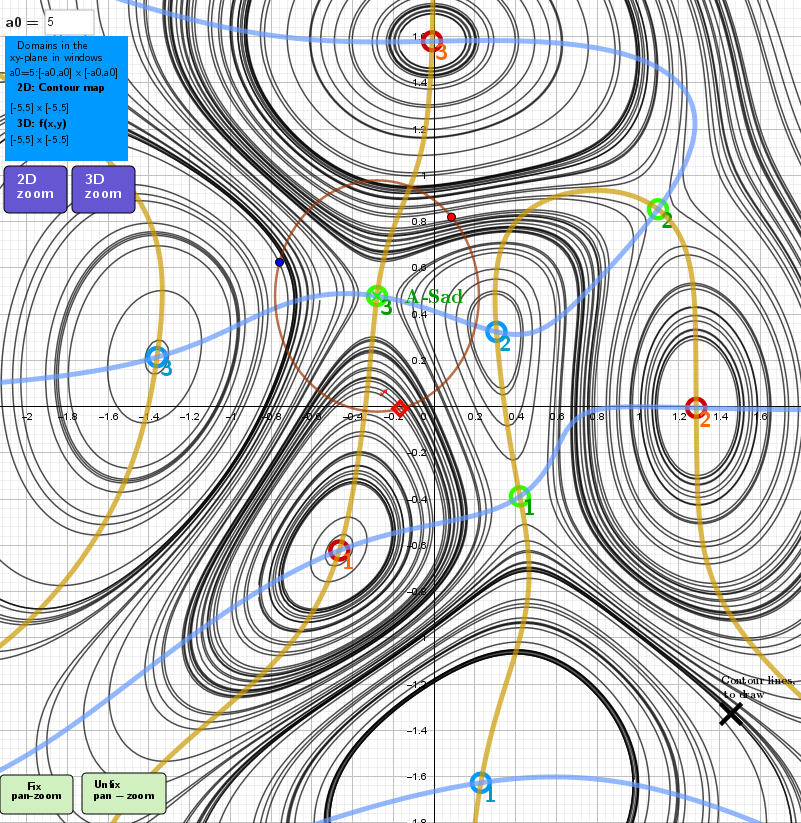
List of stationary points of the function f₄(x, y) found by CAS GeoGebra:
Local maximum points➟
{(-0.4655263056553, -0.6217120029846), (1.285162657453, -0.004833795524588), (-0.01059996592404, 1.580343715217)};
Local minimum points➟
{(0.2288469494985, -1.626050253893), (0.3052469976531, 0.3238381792756), (-1.35971813141, 0.2144664990768)};
Saddle points➟
{(0.4203044911699, -0.3877541612692), (1.097503671463, 0.8540090517851), (-0.2806862254121, 0.4785049750475)}}.
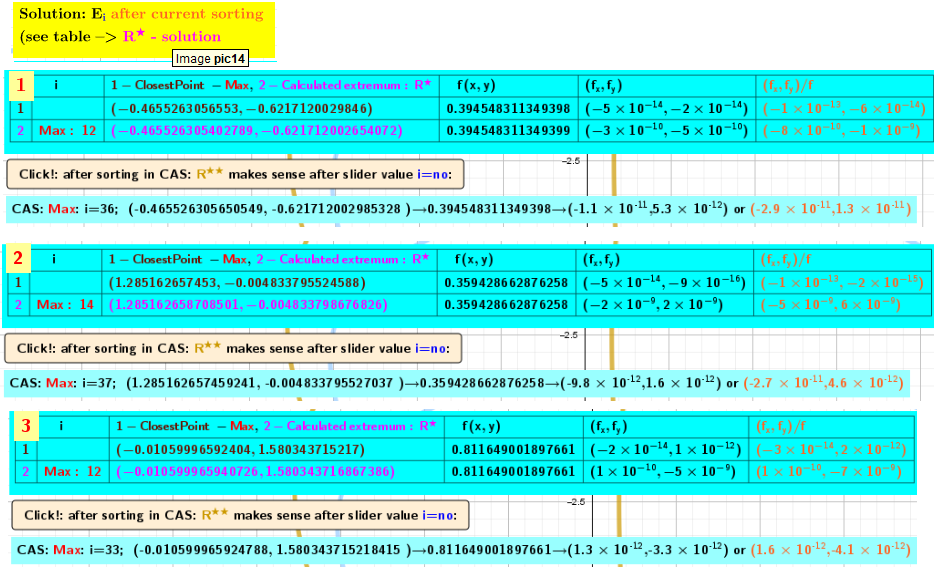
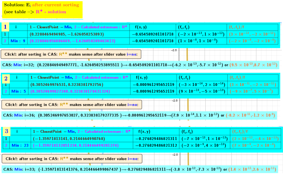
Two independent methods compare the coordinates of possible local extrema (here -Closes Points), function values, and the corresponding values of partial derivatives (which should be zero) at these points.
-In the first method (1), the calculation was performed using CAS GeoGebra based on the knowledge of the partial derivatives.
-In the second method (2), the calculations are performed using my proposed algorithm: Descent-ascent numerical method for finding the stationary points of a function of two variables without using its derivatives.
In the tables, in the second row, you can see the iteration number whose coordinates correspond to the local maximum or minimum. Due to the fact that the function values at points no+2 of the iterations are almost identical within the accuracy of the GeoGebra algebra. For this reason, the calculations were duplicated by sorting close function values using CAS, where the accuracy of the calculations is much higher.
To calculate saddle points, di - the distance between two characteristic points for each iteration - was chosen as a criterion. The iteration is considered optimal if this distance is minimal. These distances for different iterations differ enough that the calculations can be done without using CAS.
Calculated points of Local maxima
Calculated points of Local minima
Calculated Saddle Points
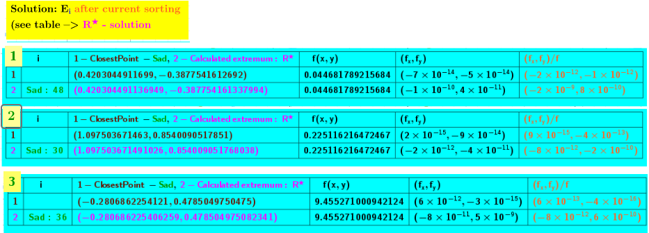
Obviously, the relative error (fx,fy)/f of partial derivatives of the first CAS -method(1) is very small. The accuracy of the calculations using the proposed method (2) for all types of local extrema is also quite high, as can be seen from the tables.