Algorithm for finding the location of the expected saddle point of stationary points of a function of two variables in the coordinate descent-ascent method
Algorithm for finding the location of the expected saddle point of stationary points of a function of two variables in the coordinate descent-ascent method
I used
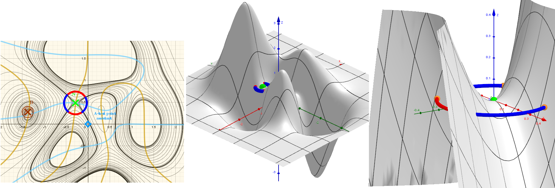
- contour map or heat map to approximate the location of stationary points for a function of two variables,
- GeoGebra Maximize/Minimize commands and the coordinate ascent/descent method. The iterative method for finding stationary points for cases of saddle points was developed by me - I did not find corresponding numerical methods in the literature.
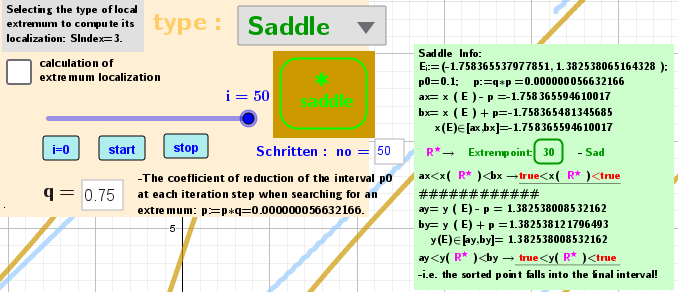
At each iteration step we have a new point Ei+1, and then the interval of change around the new point decreases ↘: [x(Ei)-p, x(Ei)+p] and correspondingly [y(Ei)-p, y(Ei)+p]. p is the radius of the circle described around new point E. po is the initial radius, then it decreases according to the law p:=p*q. My q=0.75.
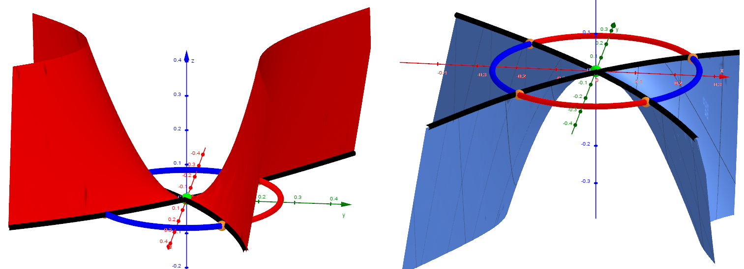
A saddle point, which seems to divide a function into two halves of growth ↗ and decrease ↘ of the function.
➤On the contour map, we draw a circle with the center E at the point of the selected initial approximation of the saddle point search and with a radius p, which is initially an iterative process p0 and then gradually decreases ↘ according to a preselected law.
➤On this circle we will find characteristic points B01 and B02: the maximum value a1 of the function (using the Maximize command) and the minimum value (again a1) of the function (using the Minimize command). Here we will assume that on the circle, symmetrically with respect to the center of the circle, these points have "doubles" - points B1 and B2 also of the maximum and minimum values of the function. In the direction of the largest values of the function it increases ↗, and in the direction of the smallest values it decreases ↘.
➤Iteration Cycle: : Let's connect these point pairs of "hot" and "cold" points with segments f1 and f2. First, along the first segment f1 we find the coordinates of the point with the minimum value a1 of the function - it is a new position (E) of the saddle point U1. Again, on the newly drawn circle, we find the coordinates of the point B02 of the smallest values a1 of the function and, accordingly, its "double" B2. We will connect the "cold" points with the segment f2 and find the coordinates of the point U2 where the function takes the maximum value. This will be the new position E of the saddle point.
We repeat this cycle many times in the "hope" that the centers of these segments should coincide. Convergence is always in question!
 |
|

The iterative cycle under consideration turned out to be productive. Evaluation As calculations have shown, the algorithm using only the U1 or only the U2 sequence has poor convergence.
To calculate saddle points, di - the distance between two characteristic points U1 and U2 for each iteration - was chosen as a estimated parameter. After no+2 iteration steps, the smallest one is selected from all these estimated parameters. These distances are sufficiently different for different iterations that the calculations can be done in the GeoGebra algebra without using CAS.
An example of such a calculation is given here.
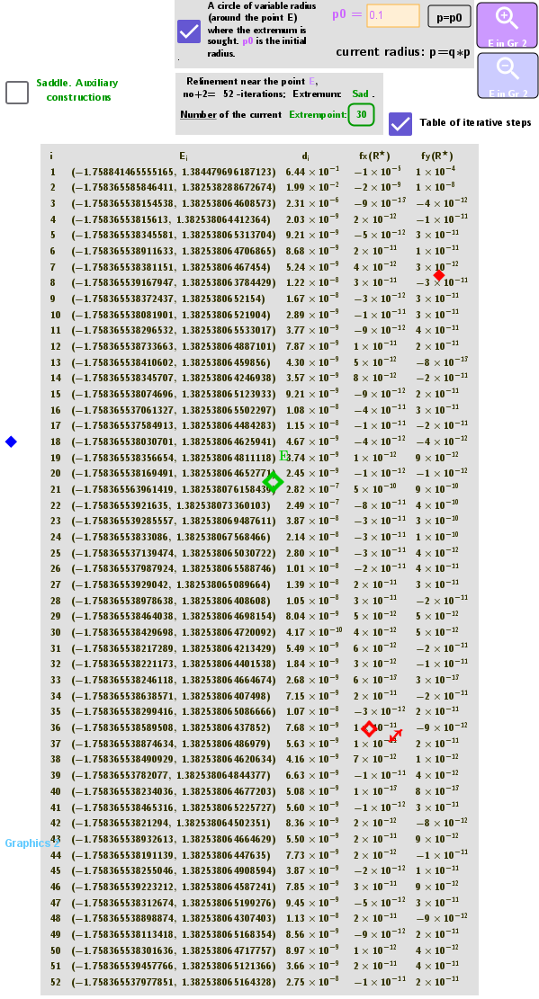
![[size=85] [b][color=#980000]ClosestPoint[/color][/b] is a [b][color=#6aa84f]saddle point[/color][/b] found earlier using [b]CAS[/b]. [b]f[sub]x[/sub][/b] and [b]f[sub]y[/sub][/b] are partial derivatives at this [b][color=#980000]point [/color][/b]and at the [color=#ff00ff][b]point[/b][/color] found by the proposed method. Here it is iteration [b][color=#6aa84f]30[/color][/b] in the list above. For stationary points, these derivatives are zero. As can be seen, the iterative calculations are performed with a high degree of accuracy. [color=#ff7700][b](f[/b][sub]x[/sub][b],f[/b][sub]y)[/sub][/color][b][color=#ff7700]/f [/color]-[/b][color=#333333]We consider it as a "relative" error.[/color][/size]](https://www.geogebra.org/resource/kzfswt7x/AN470Qi82oft5B0a/material-kzfswt7x.png)